Deep Learning for Audio Classifcation of Wildlife Vocalizations

Passive Acoustic Monitoring allows researchers to get in-depth biodiversity data faster than ever before.
Overview
Deep learning refers to a subset of machine learning that employs artificial neural networks with multiple layers to progressively extract higher-level features from raw input. In simpler terms, deep learning can be understood as a way for a computer to learn and make decisions by itself, similarly, in some ways, to the way a human brain does. Instead of neurons, though, neural networks use a series of interconnected layers in a network to analyze and interpret data.
These models, particularly the Convolutional Neural Networks (CNNs) that I am going to talk about here–are excellent at processing audio data–enabling automatic learning of intricate patterns in the sound, which is crucial for tasks like voice recognition, sound classification, and audio event detection.
Why are they so good at this?
One major strength of neural networks, particularly CNNs, lies in their ability to work with raw inputs without explicit instructions from data scientists about what specific features to look for. This is a significant advantage because it allows the model to autonomously identify relevant features that might not be immediately obvious or known to humans. Traditional machine learning models often require the data scientist to extract features manually, making their own choices about what acoustic properties they think will be important for downstream tasks such as classification.
During the training process, the neural network adjusts its numerous parameters (often in the millions) to better represent the data it’s learning from. This process is essentially the model learning to identify and prioritize the most important features in the audio to perform the task at hand: as the data passes through this complex network, each node takes on a different value that impacts how the output at each layer is transformed. The downside of this is that it is often quite difficult for us find out what those features are since the models themselves are so complex and the latent representations it has built within this intricate network of nodes are not directly retrievable. So, while traditional ML models that rely on manual feature extraction might provide greater interpretability–i.e., you can directly see which extracted features were the most important for the classification decision–deep learning models forego this interpretability but key into intricate patterns that would have otherwise been impossible to explicitly extract by dramatically increasing the scale of learnable parameters.
How do they work?
Transforming audio into a spectrogram
The preprocessing stage will vary from project to project, but a common preprocessing step involves transforming the raw audio into a two-dimensional array called a spectrogram.
A spectrogram, like the ones pictured below, visually shows how the spectrum of frequencies in the sound varies with time. In these arrays, the y-axis represents frequency, the x-axis represents time, and the intensity of color or shade in the image represents the amplitude of the sound at any given frequency at any given time.
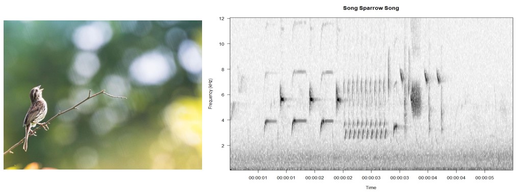
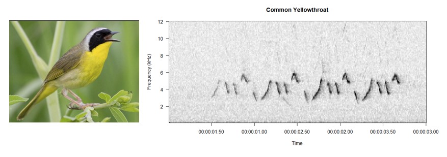
The spectrograms and associated audio clips of a song sparrow and a common yellowthroat song. Note how the variations in sound are represented visually. Effectively, models trained to analyze these visual representations are picking up on fine-grained elements of the original sound.
Another benefit of using spectrograms is the dimensionality reduction that occurs during the transformation. Raw audio samples, especially from recordings with high sample rates, are often very large, so the transformation to a spectrogram not only highlights important features, but it does so while still being able to reduce the overall size of data you have to pass through your model.
While there are numerous other steps often taken during preprocessing before the final spectrogram is passed to the model for training, what’s important for the purposes of this article is simply understanding that in this early stage, the audio is transformed into an image of itself that highlights key features. From the perspective of the model, these images are just two-dimensional arrays of numbers.
How CNNs process audio/image data
The core feature that makes CNNs so effective for these tasks is their convolutional layers. Let’s break down how these layers work and why they are beneficial.
Convolutional Layers
- The primary building blocks of CNNs are the convolutional layers. These layers use filters or kernels to scan over the input data (like images or spectrograms) in small sections at a time (see GIF below).
- As the filter moves across the input, it performs element-wise multiplication with the part of the image it’s covering and sums up the results. This process effectively extracts features such as edges, textures, or specific patterns from the input data.
Feature Learning
- Each filter in a convolutional layer learns to detect a specific type of feature in the input. Early layers might detect simple features like edges or colors, while deeper layers can recognize more complex patterns like simple shapes or geometrical patterns. The latest layers can then assemble these fundamental features into actual objects in the images, or in the case of the spectrograms above, the higher-level elements in a birdsong.
- This hierarchical feature learning is a key strength of CNNs. The network learns to understand the data from a low-level to a high-level perspective.
Translation Invariance
A key feature of CNNs is something called translation invariance. Once they learn a feature in one part of the image or spectrogram, they can recognize it in any other part. This helps a lot in audio classifcation where a birdsong, for example, could occur at various time steps within the frame or at slightly higher or lower frequencies. In image classification, this is also crucial because it means that it can learn, e.g., what an ‘eye’ is, and then apply that learning to any other eye it sees no matter where it occurs within the image.
Fully Connected Layers
- After the convolutional layers (which are often interspersed with other elements, such as pooling layers which help reduce dimensionality and features like skip-connections in the case of ResNets), the model then passes this learned representation of the audio/image to its fully connected layers for classification. These are densely connected layers that look at what the model has passed it and assign a predicted label.
Model Training
During training, the model uses the above process to analyze spectrograms and assign a predicted label. At first, of course, these predictions are wild guesses, because the model has no idea what it is looking for. Because the training dataset is labelled, the model has the ability to check if it was correct. A loss function is used to calculate the degree to which it missed its mark, and the model then uses the feedback from the loss function to adjust its internal parameters in a way that it hopes will minimize loss on its next iteration–typically through a process called backpropagation. This adjustment aims to reduce the error in future predictions, gradually improving the model’s performance over time as it continues to learn from more data.
Hyperparameter tuning
The data scientist supervising this learning will evaluate the model’s performance and then start tuning hyperparameters in attempts to improve performance further. These hyperparameters are essentially little knobs and switches you can flip that adjust how the model learns. They include things like learning rate, a factor that controls the size of the steps the model takes when adjusting weights in each iteration; batch size, which designates how many samples the model ingests at once; the number of neurons in various layers or the number of layers, values that result in tweaks to the actual architecture of the model; and so, so many more.
The number of hyperparameters can honestly be overwhelming, and there isn’t always a clear starting point. This part of the process can be frustrating, but I love it, because it involves developing intuitions for what works and what doesn’t and there is so much room for innovation here.
Validation and test sets
During training, the a subset of the data is always withheld so that the model never sees it when making adjustments to its internal weights. Then, this validation set is used to evaluate performance at each iteration. Making sure the model performs well on this set is key, because these models will tend to memorize and overfit to their training data. What this looks like in practice is a loss value that gets increasingly smaller on the training set and larger on the validation set. This signals that the model has basically found a stable, optimal solution for the training data that does not generalize at all to new data: it has memorized what you’ve shown it. Overfitting to the validation set can also occur, however, since the data scientist is constantly tuning hyperparameters and making decisions based on the performance on the validation set. For this reason, a separate test set is often used on the final models to see how it does in the real world.
Challenges
In the real world, image and audio data is messy. In many cases, getting a deep learning model to classify clean, curated samples of audio (such as the spectrograms above or clear images of dogs and cats), has become trivial. The problem, though, is that these models need to operate well in real world, deployment environments. In the case of wildlife monitoring, this often means the audio they will be analyzing comes from low quality, continuous recordings of soundscapes that are full of ambient sound and unfamiliar, overlapping acoustic signals. These real world scenarios are the ultimate test dataset, and often there are significant performance drops between training and deployment environments.
This is where domain knowledge can really come in handy. Using knowledge of the deployment environment to inform training allows a data scientist to simulate the real world as best they can. With classifiying ecological audio, this looks like intentionally transforming your training data so that it mimics deployment conditions. I talk about this a bit more in this project post about RailNET, where I overlaid actual soundscape recordings onto my training data that came from ecoystems the model was likely to encounter. This allowed the model to practice classifying the target signal in the presence of realistic ambient sounds and vocalizations from species likely to be present during deployment.
Opportunities
There is so much potential for growth and innovation within this space. The architectures we are relying on right now may not even be relevant in a couple years. The ‘exploration’ space with different parameters and architectures is really limitless, and with so many people around the world developing these models for different purposes, it is only a matter of time before the next disruptive development that hopefully allows us to listen to our ecosystems even better!